Introduction
Modern machine learning systems rarely optimize only one clean objective. A multi-task perception model may need to segment an image, estimate depth, and predict surface normals at the same time. A graph neural network for molecular property prediction may need to predict many chemical quantities from one shared representation. A ranking system may need to balance relevance, fairness, diversity, and user satisfaction.
This is the setting of multi-objective optimization (MOO). Instead of minimizing one loss, we optimize a vector of losses:
where $\mathbf{x} \in \mathcal{D} \subseteq \mathbb{R}^d$ denotes the model parameters and $f_s$ is the $s$-th objective. In multi-task learning, each $f_s$ is often the loss of one task.
The paper PSMGD: Periodic Stochastic Multi-Gradient Descent for Fast Multi-Objective Optimization studies a practical bottleneck in this setting. Gradient manipulation methods can produce good update directions by dynamically combining task gradients, but they often pay a high computational cost at every training iteration. PSMGD asks a simple question:
If the dynamic task weights do not change much over short training intervals, do we really need to recompute them at every iteration?
The answer proposed in the paper is no. PSMGD computes dynamic weights periodically, reuses them between recomputation steps, and still preserves strong convergence guarantees.
Paper links:
- Paper HTML: ar5iv version
- Extended version: arXiv:2412.10961
- Proceedings version: AAAI 2025
- Code: MarcuXu/PSMG
Before going into the algorithm, it helps to separate three layers of the problem:
- The learning setting: one model is trained against several losses, usually because the model must serve several tasks or satisfy several evaluation criteria.
- The optimization target: there is usually no single point that minimizes every loss at the same time, so the goal becomes finding a good trade-off or a Pareto-stationary point.
- The computational bottleneck: adaptive MOO methods often need multiple task-gradient computations and an extra weighting step, which is much more expensive than ordinary single-loss SGD.
PSMGD mainly attacks the third layer. It does not claim that multi-objective learning can avoid trade-offs. Instead, it asks whether the expensive part of gradient-aware trade-off negotiation has to happen at every single iteration.
This distinction is important because MOO papers often mix two different questions. The first question is preference modeling: which trade-off among objectives does the user actually want? The second question is training mechanics: given a trade-off rule, how expensive is it to produce a useful update direction? PSMGD mostly belongs to the second category. It assumes we still want a gradient-aware update, but it tries to make that update cheaper in the stochastic deep-learning loop.
In modern multi-task learning, this cost difference can dominate the method choice. A single shared backbone may be followed by many task heads, and each task loss may require a separate backward pass if the method needs exact per-task gradients. For small academic examples this overhead is manageable. For large vision backbones, graph networks, or dense prediction systems, repeatedly materializing all task gradients can become the main training bottleneck.
Why Multi-Objective Optimization Is Hard
The most direct way to handle multiple losses is linear scalarization:
This converts MOO into a standard single-objective problem. It is computationally cheap because one weighted loss can be backpropagated once.
The weakness is that fixed weights can behave poorly when task gradients conflict. Let $\nabla f_i(\mathbf{x})$ and $\nabla f_j(\mathbf{x})$ be two objective gradients. If their inner product is negative,
then moving in the direction that helps one objective may hurt the other. This is common in multi-task learning: improving one task’s loss can temporarily damage another task’s loss.
The more principled target is not a single optimum for one scalar loss, but a Pareto stationary point. A point $\mathbf{x}$ is Pareto stationary when the following common-descent condition is impossible:
This condition is important because exact Pareto optimality is generally too hard to seek directly in large non-convex models. Pareto stationarity is a practical first-order goal.
The Standard Gradient-Manipulation View
Multiple Gradient Descent Algorithm (MGDA) is a useful reference point. Given the gradients of all objectives, MGDA finds a convex combination with minimum norm:
The gradient-combination vector is then
The actual descent step moves along $-\mathbf{d}$. If $\mathbf{x}$ is not Pareto stationary, this type of combined gradient can induce a common descent direction. This is the main strength of gradient manipulation methods: they adapt weights according to the current gradient geometry rather than relying on static hand-tuned coefficients.
The cost is the extra dynamic-weight computation. In many deep-learning systems, one must compute or approximate each task gradient, solve an additional optimization problem, combine the gradients, and then update the model. This can become expensive when:
- the number of objectives $S$ is large,
- the model dimension $d$ is large,
- the method recomputes dynamic weights at every iteration,
- the training loop is already bottlenecked by backpropagation.
This is the bottleneck PSMGD targets.
Related Work Context
The simplest baseline for MOO is static scalarization, where the user fixes $\lambda_s$ before training. It is cheap and easy to implement, but it cannot react when tasks conflict or when one task learns much faster than another.
Uncertainty weighting, GradNorm, and other loss-balancing methods try to make scalarization less brittle by adapting task weights from loss scale, training speed, or uncertainty. These methods are usually easier to run than full gradient manipulation, but their update rule may not directly reason about gradient conflict. They can balance magnitudes without necessarily finding a common descent direction.
MGDA improves on this by choosing the convex combination of gradients with minimum norm. It is a natural first-order method for Pareto stationarity, but it needs the current gradients of all objectives whenever the weights are recomputed. This makes MGDA a strong conceptual baseline and also a useful way to see the cost problem: the method is principled, but its per-iteration expense grows with the number of objectives.
Later multi-task and MOO methods modify this basic idea in different ways. PCGrad projects away pairwise conflicting gradient components. CAGrad seeks a direction that balances average training progress and conflict control. IMTL-G, NashMTL, FAMO, FairGrad, and related dynamic-weighting methods all try to improve the trade-off between task balance, stability, and final quality.
These methods can be grouped by what they consider expensive. Projection methods focus on modifying the gradient after conflicts are detected. Game-theoretic and fairness-driven methods focus on choosing a more balanced update rule. Online dynamic-weighting methods focus on making the weight estimate stable during stochastic training. PSMGD cuts across these groups because it can be paired with different dynamic-weight calculators; the main scheduling idea is to amortize the calculator over several ordinary update steps.
PSMGD is best understood as complementary to this line of work. Its key question is not only “which dynamic weighting rule should we use?”, but also “how often do we need to pay for that rule?” The paper therefore focuses on periodic reuse: compute an adaptive weight vector occasionally, keep using it while it remains useful, and reduce the number of expensive all-task-gradient calculations.
The Key Observation Behind PSMGD
The paper’s core observation is empirical and algorithmic:
Dynamic weights often change slowly over short intervals.
In the pedagogical Fonseca example, MGDA’s dynamic weights converge quickly and then stay stable. In the paper’s multi-task learning studies, the same idea appears at both epoch and iteration scales: the average dynamic weights are stable and show low variability.
This suggests that recomputing $\boldsymbol{\lambda}_t$ at every iteration may be wasteful. If the current dynamic weights are close to the previous dynamic weights, we can reuse the old weights for several iterations and spend the saved computation on actual model updates.
This is the central design idea of Periodic Stochastic Multi-Gradient Descent (PSMGD).
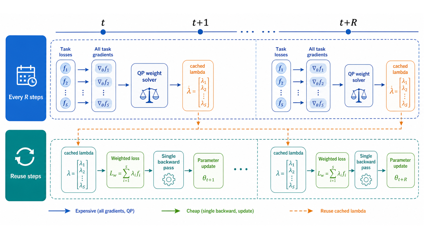
The diagram highlights the practical asymmetry between the two step types. A calculation step pays for all task gradients and solves the dynamic-weight problem. A reuse step keeps the cached weights, forms the weighted loss, and can run a single ordinary backpropagation before the model update.
The important mechanism is the cached weight vector $\boldsymbol{\lambda}$. It turns the training loop into alternating phases: a coordination phase, where objectives negotiate through all-task gradients, and a production phase, where the model uses the latest negotiated weights for cheaper stochastic updates. The period $R$ controls how long the production phase lasts before the next coordination phase.
Algorithmic Architecture
PSMGD has three moving parts:
- Periodic weight calculation: every $R$ iterations, solve the dynamic-weight problem.
- Weight smoothing: mix the newly computed weights with the previous periodic weights.
- Weight reuse: between periodic calculation steps, reuse the most recent weights and train with a weighted loss.
The architecture can be read as:
Objective losses f_1, ..., f_S
        |
        v
At t % R == 0: compute all task gradients
        |
        v
Solve dynamic-weight QP for lambda_hat_t
        |
        v
Momentum smoothing: lambda_t = alpha_t lambda_{t-R} + (1 - alpha_t) lambda_hat_t
        |
        v
Reuse lambda_t for intermediate iterations
        |
        v
Weighted loss or weighted gradient using cached lambda_t
        |
        v
Parameter update x_{t+1} = x_t - eta_t d_t
More formally, when $t \bmod R = 0$, PSMGD computes:
Here $\xi_t$ denotes the stochastic mini-batch randomness. The computed weights are then smoothed:
At the first periodic calculation step, this can be implemented by setting $\alpha_t = 0$ or by initializing the previous weight vector to a valid simplex point such as uniform weights. The important point is that the first usable dynamic weight vector must be well-defined before reuse begins.
When $t \bmod R \ne 0$, PSMGD simply reuses the previous weights:
Finally, it constructs the stochastic common direction:
and updates the parameters:
This is a small change in code structure but a large change in computational behavior. Most iterations no longer need to solve the dynamic-weight problem. More importantly for deep learning, reuse iterations can be implemented as an ordinary backward pass through the weighted loss $\sum_s \lambda_{t,s} f_s(\mathbf{x}_t,\xi_t)$, instead of computing and storing every per-objective gradient just to decide the weights again.
Pseudocode
Input: initial parameter x_0, learning rates eta_t, period R
Initialize lambda_0, or use alpha_t = 0 at the first calculation step

for t = 0, 1, ..., T - 1:
    if t mod R == 0:
        compute stochastic gradients grad f_s(x_t, xi_t) for all objectives
        solve the MGDA-style quadratic problem to obtain lambda_hat_t
        if this is the first calculation step, set alpha_t = 0
        lambda_t = alpha_t lambda_{t-R} + (1 - alpha_t) lambda_hat_t
    else:
        lambda_t = lambda_{t-1}

    form the weighted loss or weighted stochastic gradient using lambda_t
    d_t = sum_s lambda_{t,s} grad f_s(x_t, xi_t)
    x_{t+1} = x_t - eta_t d_t
The hyperparameter $R$ controls the trade-off:
- $R=1$ resembles standard dynamic gradient manipulation with frequent weight updates.
- Larger $R$ reduces dynamic-weight computation.
- If $R$ is too large, the reused weights may become stale.
The main symbols are:
- $S$: number of objectives or tasks.
- $R$: period for recomputing the dynamic weights.
- $\eta_t$: learning rate at iteration $t$.
- $\boldsymbol{\lambda}_t$: objective-weight vector used at iteration $t$.
- $\alpha_t$: momentum coefficient for smoothing newly computed weights.
- $\xi_t$: stochastic mini-batch randomness.
The algorithm is therefore best understood as a principled “lazy update” scheme for multi-objective gradient weights.
Why Reusing Weights Can Still Work
The risk of reusing $\boldsymbol{\lambda}$ is that the training landscape changes while the weights stay fixed. The paper handles this by analyzing two cases:
- Calculation steps, where the current stochastic gradients influence the newly computed weights.
- Reuse steps, where the weights are fixed from previous steps and are independent of the current mini-batch sampling.
This distinction matters because the stochastic analysis is different in the two cases. At calculation steps, the weight vector depends on the same stochastic gradients used in the update. At reuse steps, the weight vector behaves like a fixed coefficient vector for the current stochastic gradient estimate.
The paper defines the weighted objective:
with gradient:
The convergence analysis then studies progress under common assumptions such as smoothness, bounded stochastic-gradient variance, bounded weights, and bounded gradients.
At a high level, the theory says:
- For strongly convex objectives, PSMGD reaches an $\mathcal{O}(1/T)$ convergence rate.
- For general convex objectives, PSMGD reaches an $\mathcal{O}(1/\sqrt{T})$ rate.
- For non-convex objectives, PSMGD also reaches an $\mathcal{O}(1/\sqrt{T})$ stationarity-style rate.
These match state-of-the-art iteration rates for stochastic MOO methods, while reducing the number of expensive dynamic-weight computations.
Backpropagation Complexity
Iteration complexity alone is not enough for MOO. Two methods can have the same iteration rate but very different per-iteration costs. For deep learning, the more relevant unit is often backpropagation.
The paper introduces Backpropagation Complexity (BP complexity):
the total number of backpropagation operations required to reach a specified performance threshold $\epsilon$.
This metric captures the practical cost of computing per-objective gradients. PSMGD’s main efficiency result is that periodic weight calculation reduces BP complexity by a factor related to $R$.
For strongly convex functions, the paper reports:
For general convex and non-convex functions, it reports:
The interpretation is direct:
- The term involving $S$ comes from steps where all objective gradients are needed for dynamic-weight calculation.
- The term involving $R-1$ comes from reuse steps, which behave more like a weighted single-objective update.
- Increasing $R$ amortizes the expensive all-objective gradient computation.
Most importantly, if $R = \Omega(S)$, the BP complexity becomes objective-independent in order:
and
This is the most important theoretical message of the paper: with a suitable update period, PSMGD can require the same order of backpropagation operations as classic SGD for single-objective learning.
Connection to Multi-Task Learning
In multi-task learning, a common model has shared parameters and task-specific heads. A typical training loss can be written as:
where $\theta_{\mathrm{shared}}$ denotes shared parameters and $\theta_s$ denotes task-specific parameters.
The difficult part is choosing $\lambda_s$. Static weights are simple but may ignore conflict. Fully dynamic weights are adaptive but costly. PSMGD sits between them:
- It preserves a gradient-aware dynamic weighting mechanism.
- It avoids recomputing the dynamic weights at every iteration.
- It uses periodic recomputation to keep the weights aligned with the current training state.
This makes PSMGD especially natural for deep multi-task models where the main bottleneck is repeatedly computing and manipulating multiple task gradients.
Experimental Results in Brief
The paper evaluates PSMGD mainly in multi-task learning settings, using datasets with 2 to 40 objectives:
- QM-9 for molecular property regression with 11 tasks.
- Multi-MNIST for two-task image classification.
- CelebA for 40-task facial attribute classification.
- NYU-v2 for dense prediction with segmentation, depth, and surface normal tasks.
- CityScapes for dense prediction with two tasks.
The experimental section compares PSMGD with linear scalarization and many MOO or multi-task learning baselines, including MGDA, PCGrad, CAGrad, IMTL-G, NashMTL, FAMO, FairGrad, and SDMGrad. The paper reports final task quality using two aggregate metrics:
The benchmark mix matters because different datasets stress different failure modes. QM-9 and CelebA test what happens when the number of objectives is relatively large. Multi-MNIST and CityScapes test common two-task settings where conflict is easier to inspect. NYU-v2 is especially useful because dense prediction tasks share visual structure but optimize different output spaces, so it is a realistic place for gradient conflict and task imbalance to appear.
where $M_{B,n}$ is the single-task baseline value for metric $n$, $M_{m,n}$ is method $m$’s value, and $\delta_n$ marks whether higher values are better. Lower $\Delta m%$ is better. The second metric is Mean Rank (MR), the average rank of a method across task metrics; lower MR is also better.
The main takeaway is not that PSMGD wins every single task metric. Instead, the message is more practical:
- PSMGD is competitive in final task quality and sometimes improves aggregate task metrics.
- It substantially reduces training time compared with classical gradient manipulation methods.
- It often reaches target loss thresholds earlier, especially in early training.
- It gives a strong performance-efficiency trade-off, which is exactly the design goal.
For example, on QM-9, PSMGD has the shortest total time to reach the reported average-loss thresholds, even though linear scalarization has the cheapest per-epoch cost. On NYU-v2, PSMGD has strong dense-prediction convergence behavior and reaches several task-loss thresholds fastest among the compared methods.
What I Think Is the Core Principle
The main principle behind PSMGD is:
Do expensive coordination only when it is likely to matter.
In MOO, gradient manipulation is a coordination mechanism among objectives. It decides how the objectives should negotiate an update direction. But if the negotiation result changes slowly, then renegotiating every iteration is unnecessary.
PSMGD exploits this temporal structure. It does not discard dynamic weighting; it schedules it. This is why the method is simple but meaningful: it respects the geometry of multi-objective descent while reducing redundant computation.
There is also a broader lesson for optimization algorithm design. A method can be theoretically elegant but practically slow if it optimizes the wrong unit of cost. PSMGD explicitly shifts attention from iteration count to backpropagation count, which is closer to the real cost in deep learning.
Limitations and Open Questions
PSMGD introduces the period hyperparameter $R$, and this choice matters. If $R$ is too small, the method approaches ordinary dynamic gradient manipulation and saves less computation. If $R$ is too large, the reused weights may become stale and less aligned with the current gradients.
The method also assumes that dynamic weights are sufficiently stable over short intervals. This is often reasonable in the studied settings, but it may be less reliable in highly non-stationary training regimes, rapidly changing curricula, reinforcement learning, or tasks whose losses change at very different speeds.
Another practical issue is that the best period may change during training. Early iterations can have unstable gradients and rapidly changing task relationships, while later iterations may have smoother weight trajectories. A fixed $R$ is simple and analyzable, but an adaptive schedule could update more often during unstable phases and reuse weights more aggressively once the task geometry becomes steadier.
Several natural extensions follow:
- Adaptive period selection: update weights when gradient conflict changes enough, not only every fixed $R$ steps.
- Preference-aware PSMGD: combine periodic weighting with user-specified trade-off preferences.
- Pareto set learning: use the efficiency gain to explore multiple trade-off solutions rather than one solution.
- Distributed or federated MOO: reduce communication and backpropagation cost when many objectives or clients are involved.
Takeaways
PSMGD is built around a clean observation: dynamic MOO weights are often stable enough to reuse. By periodically computing gradient-aware weights and reusing them between updates, the method preserves the benefits of gradient manipulation while reducing its most painful computational overhead.
The paper’s central contributions are:
- a periodic stochastic multi-gradient algorithm for fast MOO,
- convergence guarantees for strongly convex, convex, and non-convex objectives,
- a BP complexity metric that better reflects deep-learning training cost,
- objective-independent BP complexity when $R$ scales with the number of objectives,
- empirical evidence that the method improves the performance-time trade-off in multi-task learning.
In one sentence: PSMGD makes multi-objective gradient manipulation more practical by realizing that task-weight negotiation does not need to happen at every step.